Spline SPF Injection-Recovery

This notebook demonstrates injection-recovery for a flexible spline scattering phase function (SPF) in GRaTeR-JAX.

In scattered-light imaging of debris disks, the scattering phase function (SPF) encodes how dust grains scatter starlight as a function of the angle between the incident and scattered rays. Recovering the SPF from disk images constrains dust grain properties — size, composition, and porosity — that are otherwise inaccessible.

GRaTeR-JAX supports a flexible spline SPF that can represent arbitrary shapes, unlike the single-parameter Henyey-Greenstein (HG) model. The spline is parameterised by a small number of free knot values, making it tractable for both maximum-likelihood optimisation and Bayesian MCMC posterior inference.

Injection-recovery is a standard validation strategy: we synthesise a disk image using a known SPF (here, a HG with $g = 0.3$), then attempt to recover the SPF using the flexible spline model. Agreement between the recovered and injected SPF validates the modelling pipeline and quantifies the recovery fidelity.

This notebook will:

Generate truth images at four disk inclinations (30°, 50°, 70°, 80°).
Fit the spline SPF to each truth image with scipy L-BFGS-B optimisation.
Run MCMC posterior inference with emcee to quantify uncertainty on the recovered SPF.
Summarise the recovery fidelity across inclinations.

Background

Henyey-Greenstein SPF

The Henyey-Greenstein (HG) phase function is the standard single-parameter model for dust scattering:

\[f(\theta) = \frac{1}{4\pi}\frac{1-g^2}{[1+g^2 - 2g\cos\theta]^{3/2}}\]

where $\theta$ is the scattering angle and $g \in (-1, 1)$ is the asymmetry parameter ($g > 0$ forward-scattering, $g < 0$ backward-scattering, $g = 0$ isotropic). While analytically convenient, the HG model has only one free parameter and cannot reproduce the rich scattering behaviour of real grain populations.

Spline SPF

The spline SPF replaces the analytic HG formula with a cubic spline interpolated over $N_k$ free knot values across the probed range of $\cos\phi$ (where $\phi$ is the scattering angle). This gives much greater flexibility:

Knot locations are evenly distributed across the range of $\cos\phi$ probed by the disk geometry, plus a small buffer (KNOT_BOUND_BUFFER = 0.1 in $\cos\phi$ units) beyond the probed range.
A fixed knot is always placed at :math:`cosphi = 0` (90°) with value 1. This normalisation means the spline value at 90° is always 1, so the absolute flux scaling (flux_scaling) and the SPF amplitude are not degenerate. All SPF comparisons in this notebook are therefore on a normalised scale.
Free knot values (the $N_k$ parameters to be optimised) are the spline values at all positions except the fixed centre knot.

Angular coverage and the inclination limit

A disk at inclination $i$ probes scattering angles from approximately $90° - i$ to $90° + i$ (forward to backward). Equivalently, the probed range in $\cos\phi$ is $(-\sin i, +\sin i)$. At low inclinations this window is narrow, and the spline has little angular leverage. The recommended_num_knots utility scales $N_k$ with the probed window, with a minimum of 4 (fewer knots leads to underdetermined systems and local-minimum failures). Below roughly 28°, the error on the SPF is large and the minimization may not converge. At very high inclinations, there is an inherent degeneracy as the SPF is being probed at multiple scattering angles for each line of sight.

Injection-recovery as validation

We synthesise a truth image $I_{\rm true}$ from a known HG SPF, then attempt to recover it with the spline model. Any discrepancy between the recovered spline and the true HG reveals either (a) degeneracies in the model, (b) fitting failures, or (c) intrinsic limits set by the angular coverage.

Setup

[1]:

import os
import numpy as np
import matplotlib.pyplot as plt
import matplotlib.gridspec as gridspec
import jax
import jax.numpy as jnp
import emcee

# Enable 64-bit precision for numerical stability in optimization and MCMC
jax.config.update("jax_enable_x64", True)
# Limit JAX memory fraction to leave room for other processes
os.environ["XLA_PYTHON_CLIENT_MEM_FRACTION"] = "0.5"

from grater_jax.disk_model.SLD_ojax import ScatteredLightDisk
from grater_jax.disk_model.SLD_utils import (
    DustEllipticalDistribution2PowerLaws,
    HenyeyGreenstein_SPF,
    InterpolatedUnivariateSpline_SPF,
    recommended_num_knots,
)
from grater_jax.disk_model.objective_functions import Parameter_Index
from grater_jax.optimization.optimize_framework import Optimizer

All constants are collected in one place below. Keeping magic numbers here (rather than scattered through code) makes it easy to re-run the notebook with different configurations.

[2]:

# ── True SPF parameters ───────────────────────────────────────────────────────
G_TRUE    = 0.3          # true HG asymmetry parameter
INIT_G    = 0.5          # assumed g for initialising spline knots (not a constraint)

# ── Disk / image setup ────────────────────────────────────────────────────────
NX, NY    = 140, 140
FLUX      = 1e6
NUM_KNOTS = 6            # requested knot count for full angular range
FIT_ITERS = 2000

# ── Knot placement ───────────────────────────────────────────────────────────
KNOT_BOUND_BUFFER = 0.1  # cos(φ) buffer beyond probed range for knot boundaries

# ── Inclinations to test ──────────────────────────────────────────────────────
INCLINATIONS = [30.0, 50.0, 70.0, 80.0]

# ── MCMC settings ─────────────────────────────────────────────────────────────
NWALKERS  = 64
NITER     = 2000
BURNS     = 200
MCMC_DIR  = "mcmc_backends"

# ── Convenience: HG value at 90° (cos φ = 0); used for flux initialisation ───
# The spline SPF is normalised to 1 at 90°, so flux_scaling must absorb
# the HG value at that angle to produce the correct total flux.
# Note that this is
hg_at_90  = float((1.0 / (4.0 * np.pi)) * (1 - G_TRUE**2) / (1 + G_TRUE**2)**1.5)

# ── Base parameter dictionaries ───────────────────────────────────────────────
BASE_MISC = Parameter_Index.misc_params.copy()
BASE_MISC.update({
    "nx": NX, "ny": NY,
    "distance": 50.0,
    "pxInArcsec": 0.01225,
    "halfNbSlices": 25,
    "flux_scaling": FLUX,
})

BASE_DISK = Parameter_Index.disk_params.copy()
BASE_DISK.update({
    "sma": 46.0, "alpha_in": 5.0, "alpha_out": -5.0,
    "ksi0": 1.0, "gamma": 2.0, "beta": 1.0,
    "e": 0.0, "dens_at_r0": 1.0,
    "position_angle": 0.0, "omega": 0.0,
    "x_center": NX / 2, "y_center": NY / 2,
    "halfNbSlices": 25,
})

HG_SPF_PARAMS = HenyeyGreenstein_SPF.params.copy()
HG_SPF_PARAMS["g"] = G_TRUE

[3]:

def hg_normalized(cos_phi, g):
    """HG SPF normalised to 1 at cos_phi=0 (scattering angle = 90°)."""
    raw  = (1.0 / (4.0 * np.pi)) * (1 - g**2) / (1 + g**2 - 2*g*cos_phi)**1.5
    norm = (1.0 / (4.0 * np.pi)) * (1 - g**2) / (1 + g**2)**1.5
    return raw / norm


def probed_cosphi_range(incl_deg):
    """cos(φ) range probed by a disk at the given inclination: (−sin i, +sin i)."""
    s = np.sin(np.radians(incl_deg))
    return -s, s


# Dense grid for evaluating SPF curves
cos_grid = np.linspace(-1.0, 1.0, 500)
angles   = np.degrees(np.arccos(cos_grid))   # scattering angle in degrees

The True SPF and Angular Coverage

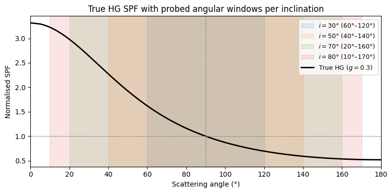
Before fitting anything, it is instructive to visualise (a) the true HG SPF and (b) the range of scattering angles that each disk inclination actually probes. The shaded grey regions below fall outside the probed range — the spline has no direct data constraint there, and any apparent agreement is due to extrapolation only.

[4]:

true_spf_curve = hg_normalized(cos_grid, G_TRUE)

fig, ax = plt.subplots(figsize=(8, 4))

colors = ["C0", "C1", "C2", "C3"]

for incl, col in zip(INCLINATIONS, colors):
    cp_back, cp_fwd = probed_cosphi_range(incl)
    ang_fwd  = float(np.degrees(np.arccos(cp_fwd)))
    ang_back = float(np.degrees(np.arccos(cp_back)))
    # Shade the probed region (not grayed out)
    ax.axvspan(ang_fwd, ang_back, alpha=0.12, color=col,
               label=f"$i={incl:.0f}$° ({ang_fwd:.0f}°–{ang_back:.0f}°)")

ax.plot(angles, true_spf_curve, "k-", lw=2, label=f"True HG ($g={G_TRUE}$)")
ax.axvline(90, color="grey", ls="--", lw=0.8)
ax.axhline(1.0, color="grey", ls="--", lw=0.8)

ax.set_xlabel("Scattering angle (°)")
ax.set_ylabel("Normalised SPF")
ax.set_title("True HG SPF with probed angular windows per inclination")
ax.set_xlim(0, 180)
ax.legend(loc="upper right", fontsize=9)
plt.tight_layout()
plt.show()

# Print probed-range table
print(f"{'Inclination':>12}  {'Probed cos-phi range':>22}  {'Probed angle range':>20}  {'Nk':>4}")
print("-" * 65)
for incl in INCLINATIONS:
    cp_back, cp_fwd = probed_cosphi_range(incl)
    ang_fwd  = float(np.degrees(np.arccos(cp_fwd)))
    ang_back = float(np.degrees(np.arccos(cp_back)))
    nk = recommended_num_knots(incl, NUM_KNOTS, boundary_buffer=KNOT_BOUND_BUFFER)
    print(f"{incl:>11.0f}°  [{cp_back:+.3f}, {cp_fwd:+.3f}]         "
          f"{ang_fwd:>6.1f}° – {ang_back:>5.1f}°          {nk:>4}")

../_images/tutorials_spline_spf_tutorial_8_0.png

 Inclination    Probed cos-phi range    Probed angle range    Nk
-----------------------------------------------------------------
         30°  [-0.500, +0.500]           60.0° – 120.0°             4
         50°  [-0.766, +0.766]           40.0° – 140.0°             4
         70°  [-0.940, +0.940]           20.0° – 160.0°             6
         80°  [-0.985, +0.985]           10.0° – 170.0°             6

Generating Synthetic Observations

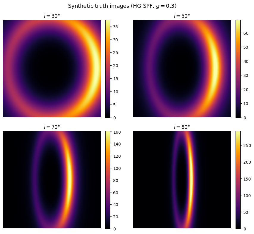
We generate a noiseless truth image using the HG SPF and create a photon-noise-like error map:

\[\sigma(x,y) = \sqrt{|I(x,y)|} \times \sqrt{I_{\rm max}} \times 0.01\]

This mimics the shape of Poisson (photon-counting) noise — pixels with more signal have larger absolute uncertainty — without requiring actual shot-noise realisations. It gives the optimiser a realistic signal-to-noise weighting without introducing stochastic variation that would make the notebook non-reproducible.

[5]:

truth_images = {}
err_maps     = {}

for incl in INCLINATIONS:
    disk_params = BASE_DISK.copy()
    disk_params["inclination"] = incl

    truth_misc = BASE_MISC.copy()
    truth_misc["flux_scaling"] = FLUX

    truth_opt = Optimizer(
        ScatteredLightDisk, DustEllipticalDistribution2PowerLaws,
        HenyeyGreenstein_SPF, None,
        disk_params, HG_SPF_PARAMS, None, truth_misc,
    )
    truth_img = np.array(truth_opt.get_model())
    err_map   = np.sqrt(np.abs(truth_img)) * np.sqrt(truth_img.max()) * 0.01

    truth_images[incl] = truth_img
    err_maps[incl]     = err_map
    print(f"incl={incl:.0f}°  truth max={truth_img.max():.4e}  err max={err_map.max():.4e}")

# ── 2×2 panel of truth images ─────────────────────────────────────────────────
fig, axes = plt.subplots(2, 2, figsize=(9, 8))
for ax, incl in zip(axes.flat, INCLINATIONS):
    img = truth_images[incl]
    vmax = np.percentile(img, 99.5)
    im = ax.imshow(img, origin="lower", cmap="inferno", vmin=0, vmax=vmax)
    ax.set_title(f"$i = {incl:.0f}$°")
    ax.axis("off")
    fig.colorbar(im, ax=ax, fraction=0.046, pad=0.04)
fig.suptitle("Synthetic truth images (HG SPF, $g=0.3$)", fontsize=13)
plt.tight_layout()
plt.show()

incl=30°  truth max=3.7960e+01  err max=3.7960e-01
incl=50°  truth max=7.1337e+01  err max=7.1337e-01
incl=70°  truth max=1.7077e+02  err max=1.7077e+00
incl=80°  truth max=3.2734e+02  err max=3.2734e+00

../_images/tutorials_spline_spf_tutorial_10_1.png

Spline Model Setup

Several design choices matter here:

``recommended_num_knots`` scales the number of knots with the probed angular window, using

\[N_k = \max\left(4,\ \text{round}\left(N_{\rm full} \cdot \frac{\text{probed window}}{2}\right)\right)\]

The minimum of 4 is enforced because fewer knots leads to an underdetermined or highly degenerate optimisation landscape with many local minima. This minimum is the reason there is a practical lower inclination limit of roughly 28°: below that, the probed window is too narrow to fit 4 knots reliably.

Knot boundary buffer of 0.1 in $\cos\phi$ places the outermost knots slightly beyond the probed range. This prevents the spline from being forced to extrapolate immediately at the boundary and generally improves numerical stability.

Extrapolation beyond inclination bounds is a straight extrapolation on the forward scattering side, to capture physically motivated forward-scattering behavior, and a constant at the backscattering side.

HG initialisation sets the starting knot values to the normalised HG curve (with $g = $ INIT_G = 0.5) evaluated at each free knot position. Starting from flat knot values (all ones) fails at low inclinations, where the narrow probed window provides only a weak gradient signal — the optimiser stalls near the flat-spline local minimum. Starting from a sensible physical shape (forward-peaked) gives a reliable warm start.

Flux scaling initialisation: Because the spline is normalised to 1 at 90°, the flux_scaling parameter must carry the physical flux value that the HG SPF had at 90°. We therefore initialise flux_scaling = FLUX * hg_at_90, where hg_at_90 is the unnormalised HG value at $\theta = 90$°. This ensures the model flux is correct from the start. This flux scaling method is specific to this synthetic injection and recovery testing. We start the flux scaling at a value close to what is known from the injected disks, as this is not intended to be a demonstration of how well the spline can be recovered from a bad choice of starting guess on flux scaling. When using real data, it is the user’s responsibility to determine a reasonable starting guess for the flux scaling based on their specific dataset.

[6]:

# Show recommended knot counts and visualise knot positions on the SPF curve
fig, ax = plt.subplots(figsize=(8, 4))
ax.plot(angles, true_spf_curve, "k-", lw=2, label=f"True HG ($g={G_TRUE}$)")

for incl, col in zip(INCLINATIONS, colors):
    cp_back, cp_fwd = probed_cosphi_range(incl)
    fwd_bound  = float(np.clip(cp_fwd  + KNOT_BOUND_BUFFER, -1.0, 1.0))
    back_bound = float(np.clip(cp_back - KNOT_BOUND_BUFFER, -1.0, 1.0))
    nk = recommended_num_knots(incl, NUM_KNOTS, boundary_buffer=KNOT_BOUND_BUFFER)

    # Build spf_params just to get knot positions
    spf_params_tmp = InterpolatedUnivariateSpline_SPF.params.copy()
    spf_params_tmp["num_knots"]          = nk
    spf_params_tmp["knot_values"]        = jnp.ones(nk)
    spf_params_tmp["forwardscatt_bound"] = fwd_bound
    spf_params_tmp["backscatt_bound"]    = back_bound

    knot_cos = np.array(InterpolatedUnivariateSpline_SPF.get_knots(spf_params_tmp))
    # Drop the fixed centre knot (cos_phi = 0) from the free-knot display
    n_left_init   = nk // 2
    free_knot_cos = np.concatenate([knot_cos[:n_left_init], knot_cos[n_left_init + 1:]])
    knot_angles   = np.degrees(np.arccos(free_knot_cos))
    knot_spf_vals = hg_normalized(free_knot_cos, G_TRUE)

    ax.scatter(knot_angles, knot_spf_vals, color=col, s=60, zorder=5,
               label=f"$i={incl:.0f}$° knots ($N_k={nk}$)")

ax.scatter([90], [1.0], marker="*", s=120, c="k", zorder=6, label="Fixed centre (90°)")
ax.axvline(90, color="grey", ls="--", lw=0.8)
ax.axhline(1.0, color="grey", ls="--", lw=0.8)
ax.set_xlabel("Scattering angle (°)")
ax.set_ylabel("Normalised SPF")
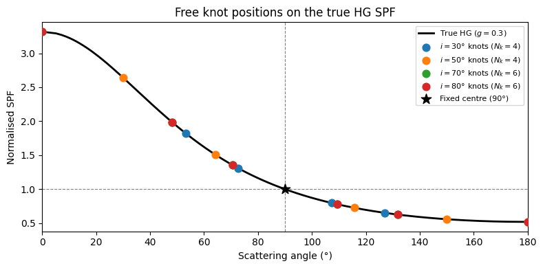
ax.set_title("Free knot positions on the true HG SPF")
ax.set_xlim(0, 180)
ax.legend(fontsize=8, loc="upper right")
plt.tight_layout()
plt.show()

print(f"{'Inclination':>12}  {'Nk':>4}  {'Notes'}")
print("-" * 50)
for incl in INCLINATIONS:
    nk = recommended_num_knots(incl, NUM_KNOTS, boundary_buffer=KNOT_BOUND_BUFFER)
    note = "(minimum; window too narrow for more)" if nk == 4 else ""
    print(f"{incl:>11.0f}°  {nk:>4}  {note}")

../_images/tutorials_spline_spf_tutorial_12_0.png

 Inclination    Nk  Notes
--------------------------------------------------
         30°     4  (minimum; window too narrow for more)
         50°     4  (minimum; window too narrow for more)
         70°     6
         80°     6

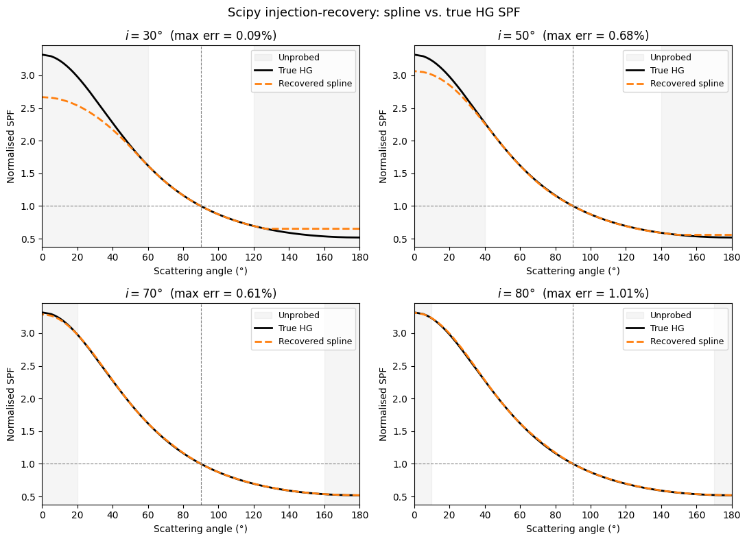
Scipy Injection-Recovery

We use L-BFGS-B bounded optimisation (via scipy.optimize.minimize) to find the maximum-likelihood spline SPF. The optimisation is run with use_grad=False, meaning finite-difference gradients rather than JAX autodiff. Tests showed identical recovery accuracy at this parameter scale (~4–6 free parameters), and finite-difference mode is faster here because the JAX JIT compilation overhead dominates for small parameter counts — the computational advantage of autodiff only exceeds JIT overhead at ~20+ free parameters.

Bounds are set to prevent nonphysical knot values: $[10^{-6}, 10^3]$ for each knot (normalised SPF value) and $[10^2, 10^{12}]$ for flux_scaling. This cell takes approximately 10–30 seconds.

[7]:

results = {}

for incl in INCLINATIONS:
    print(f"\n{'='*55}\nInclination = {incl:.0f}°")

    cp_back, cp_fwd = probed_cosphi_range(incl)
    nk          = recommended_num_knots(incl, NUM_KNOTS, boundary_buffer=KNOT_BOUND_BUFFER)
    fwd_bound   = float(np.clip(cp_fwd  + KNOT_BOUND_BUFFER, -1.0, 1.0))
    back_bound  = float(np.clip(cp_back - KNOT_BOUND_BUFFER, -1.0, 1.0))

    truth_img   = truth_images[incl]
    err_map     = err_maps[incl]

    # Build spline optimizer
    disk_params = BASE_DISK.copy()
    disk_params["inclination"] = incl

    spf_params = InterpolatedUnivariateSpline_SPF.params.copy()
    spf_params["num_knots"]          = nk
    spf_params["knot_values"]        = jnp.ones(nk)
    spf_params["forwardscatt_bound"] = fwd_bound
    spf_params["backscatt_bound"]    = back_bound

    fit_misc = BASE_MISC.copy()
    fit_misc["flux_scaling"] = FLUX * hg_at_90

    opt = Optimizer(
        ScatteredLightDisk, DustEllipticalDistribution2PowerLaws,
        InterpolatedUnivariateSpline_SPF, None,
        disk_params, spf_params, None, fit_misc,
    )

    # Warm-start knots from HG shape (avoids flat-spline local minimum at low inclinations)
    knot_cos      = np.array(InterpolatedUnivariateSpline_SPF.get_knots(opt.spf_params))
    n_left_init   = nk // 2
    free_knot_cos = np.concatenate([knot_cos[:n_left_init], knot_cos[n_left_init + 1:]])
    opt.spf_params["knot_values"]   = jnp.array(hg_normalized(free_knot_cos, INIT_G))
    opt.misc_params["flux_scaling"] = FLUX * hg_at_90

    joint_bounds = ([np.full(nk, 1e-6), 1e2], [np.full(nk, 1e3), 1e12])

    # Up to 3 passes; stop early on convergence
    for pass_num in range(1, 4):
        soln = opt.scipy_bounded_optimize(
            fit_keys=["knot_values", "flux_scaling"],
            fit_bounds=joint_bounds,
            logscaled_params=["knot_values", "flux_scaling"],
            array_params=["knot_values"],
            target_image=truth_img,
            err_map=err_map,
            use_grad=False,
            iters=FIT_ITERS,
            ftol=1e-14,
            gtol=1e-14,
        )
        status = "converged" if soln.success else soln.message[:40].strip()
        print(f"  Pass {pass_num}: nit={soln.nit}  [{status}]")
        if soln.success:
            break

    # Evaluate recovered spline on the dense grid
    spline_model = InterpolatedUnivariateSpline_SPF.pack_pars(
        opt.spf_params["knot_values"],
        knots=InterpolatedUnivariateSpline_SPF.get_knots(opt.spf_params),
    )
    recovered_spf = np.array(
        InterpolatedUnivariateSpline_SPF.compute_phase_function_from_cosphi(
            spline_model, jnp.array(cos_grid)
        )
    )

    true_spf_norm = hg_normalized(cos_grid, G_TRUE)
    in_range      = (cos_grid >= cp_back) & (cos_grid <= cp_fwd)
    frac_err      = (
        np.abs(recovered_spf[in_range] - true_spf_norm[in_range])
        / (np.abs(true_spf_norm[in_range]) + 1e-30)
    )
    max_frac_err = float(frac_err.max())
    print(f"  Max SPF error (probed range): {max_frac_err*100:.2f}%")

    results[incl] = dict(
        truth_img=truth_img,
        err_map=err_map,
        recovered_spf=recovered_spf,
        true_spf_norm=true_spf_norm,
        knot_cos=knot_cos,
        knot_values=np.array(opt.spf_params["knot_values"]),
        flux_scaling=float(opt.misc_params["flux_scaling"]),
        spline_model=spline_model,
        cp_fwd=cp_fwd,
        cp_back=cp_back,
        fwd_bound=fwd_bound,
        back_bound=back_bound,
        in_range=in_range,
        max_frac_err=max_frac_err,
        nk=nk,
    )


=======================================================
Inclination = 30°
  Pass 1: nit=26  [converged]
  Max SPF error (probed range): 0.09%

=======================================================
Inclination = 50°
  Pass 1: nit=26  [converged]
  Max SPF error (probed range): 0.68%

=======================================================
Inclination = 70°
  Pass 1: nit=31  [converged]
  Max SPF error (probed range): 0.61%

=======================================================
Inclination = 80°
  Pass 1: nit=32  [converged]
  Max SPF error (probed range): 1.01%

[8]:

# ── 2×2 SPF comparison panel ──────────────────────────────────────────────────
fig, axes = plt.subplots(2, 2, figsize=(11, 8))

for ax, incl in zip(axes.flat, INCLINATIONS):
    r = results[incl]
    ang_fwd  = float(np.degrees(np.arccos(r["cp_fwd"])))
    ang_back = float(np.degrees(np.arccos(r["cp_back"])))

    # Shade unprobed regions
    ax.axvspan(0,        ang_fwd,  alpha=0.08, color="grey")
    ax.axvspan(ang_back, 180,      alpha=0.08, color="grey",
               label=f"Unprobed")

    ax.plot(angles, r["true_spf_norm"],  "k-",  lw=2,   label="True HG")
    ax.plot(angles, r["recovered_spf"],  "--",  lw=2,   color="C1", label="Recovered spline")

    ax.axvline(90, color="grey", ls="--", lw=0.8)
    ax.axhline(1.0, color="grey", ls="--", lw=0.8)

    ax.set_xlabel("Scattering angle (°)")
    ax.set_ylabel("Normalised SPF")
    ax.set_title(f"$i = {incl:.0f}$°  (max err = {r['max_frac_err']*100:.2f}%)")
    ax.legend(fontsize=9)
    ax.set_xlim(0, 180)

fig.suptitle("Scipy injection-recovery: spline vs. true HG SPF", fontsize=13)
plt.tight_layout()
plt.show()

../_images/tutorials_spline_spf_tutorial_15_0.png

[9]:

# ── Results summary table ─────────────────────────────────────────────────────
print(f"{'Inclination':>12}  {'Probed range':>18}  {'Knots':>6}  {'Max SPF error':>14}")
print("-" * 60)
for incl in INCLINATIONS:
    r = results[incl]
    ang_fwd  = float(np.degrees(np.arccos(r["cp_fwd"])))
    ang_back = float(np.degrees(np.arccos(r["cp_back"])))
    print(f"{incl:>11.0f}°  "
          f"{ang_fwd:>6.0f}° – {ang_back:>4.0f}°  "
          f"{r['nk']:>6}  "
          f"{r['max_frac_err']*100:>12.2f}%")

 Inclination        Probed range   Knots   Max SPF error
------------------------------------------------------------
         30°      60° –  120°       4          0.09%
         50°      40° –  140°       4          0.68%
         70°      20° –  160°       6          0.61%
         80°      10° –  170°       6          1.01%

MCMC Posterior Inference

The scipy optimisation gives a point estimate of the spline SPF — the maximum-likelihood solution. To quantify uncertainty, we run Markov Chain Monte Carlo (MCMC) posterior inference using the emcee ensemble sampler.

MCMC produces a collection of samples from the posterior distribution $p(\theta | I_{\rm obs})$, where $\theta$ are the free parameters (knot values + flux scaling). From these samples we can compute:

Posterior median SPF: the point estimate from the full posterior
±1σ credible interval: the 16th–84th percentile band, showing where 68% of posterior probability lies

Setup details:

64 walkers, each starting from a small Gaussian ball around the scipy best-fit
Knot values and flux scaling are log-scaled in sampler space. This enforces positivity (log-space proposals cannot go negative) and gives better-conditioned proposal covariances, since these parameters span several orders of magnitude.
200 burn-in steps are discarded from the front of each chain
The sampler state is saved to an HDFBackend so the chain can be inspected or continued without rerunning

⏱️ Runtime warning: The MCMC cell below runs 64 walkers × 2000 steps for each of 4 inclinations. On a CPU this takes approximately 30–60 minutes. Set LOAD_MCMC_FROM_DISK = True (the default) to load from pre-computed backends instead.

[10]:

# Set to False to re-run MCMC from scratch (~30-60 min on CPU)
LOAD_MCMC_FROM_DISK = True

[11]:

os.makedirs(MCMC_DIR, exist_ok=True)

mcmc_results = {}

for incl in INCLINATIONS:
    print(f"\n{'='*55}\nInclination = {incl:.0f}°  [MCMC]")

    r  = results[incl]
    nk = r["nk"]

    backend_path = os.path.join(MCMC_DIR, f"spline_incl{int(incl):02d}_emcee_backend.h5")

    # Build the spf_params dict that defines knot positions (needed for SPF reconstruction)
    spf_params = InterpolatedUnivariateSpline_SPF.params.copy()
    spf_params["num_knots"]          = nk
    spf_params["knot_values"]        = jnp.array(r["knot_values"])
    spf_params["forwardscatt_bound"] = r["fwd_bound"]
    spf_params["backscatt_bound"]    = r["back_bound"]

    knots = InterpolatedUnivariateSpline_SPF.get_knots(spf_params)

    precomputed_path = os.path.join(MCMC_DIR, "precomputed_chains.npz")

    if LOAD_MCMC_FROM_DISK and os.path.exists(backend_path):
        # Load pre-computed chain directly from the HDF5 backend
        print(f"  Loading from {backend_path}")
        reader    = emcee.backends.HDFBackend(backend_path, read_only=True)
        flatchain = reader.get_chain(discard=BURNS, flat=True)
        # Columns: first nk are log(knot_values), last column is log(flux_scaling)
        kv_samples = np.exp(flatchain[:, :nk])   # un-log the knot values
        print(f"  Loaded {flatchain.shape[0]} posterior samples  (nk={nk})")
    elif LOAD_MCMC_FROM_DISK and os.path.exists(precomputed_path):
        # Fall back to the lightweight precomputed chains (committed to git)
        print(f"  Loading from precomputed chains ({precomputed_path})")
        precomp    = np.load(precomputed_path)
        # Values are already in real-space (exp-transformed)
        kv_samples = precomp[f"flatchain_{int(incl)}"][:, :nk]
        print(f"  Loaded {len(kv_samples)} posterior samples  (nk={nk})")
    else:
        # Run MCMC from the scipy best-fit starting point
        fit_disk = BASE_DISK.copy()
        fit_disk["inclination"] = incl

        fit_misc = BASE_MISC.copy()
        fit_misc["flux_scaling"] = r["flux_scaling"]

        opt = Optimizer(
            ScatteredLightDisk, DustEllipticalDistribution2PowerLaws,
            InterpolatedUnivariateSpline_SPF, None,
            fit_disk, spf_params, None, fit_misc,
        )
        opt.name = os.path.join(MCMC_DIR, f"spline_incl{int(incl):02d}")

        mcmc_bounds = (
            [np.full(nk, 1e-6), 1e2],
            [np.full(nk, 1e3),  1e12],
        )

        mc_model = opt.mcmc(
            fit_keys=["knot_values", "flux_scaling"],
            logscaled_params=["knot_values", "flux_scaling"],
            array_params=["knot_values"],
            target_image=r["truth_img"],
            err_map=r["err_map"],
            BOUNDS=mcmc_bounds,
            nwalkers=NWALKERS,
            niter=NITER,
            burns=BURNS,
            confirm_overwrite=False,
        )
        flatchain  = mc_model._get_flatchain(scaled=True)
        kv_samples = flatchain[:, :nk]
        print(f"  Done. Posterior samples: {flatchain.shape[0]}")

    # Reconstruct SPF curves from posterior samples
    # Subsample to 2000 curves for speed
    stride = max(1, len(kv_samples) // 2000)
    spf_samples = []
    for kv in kv_samples[::stride]:
        spline = InterpolatedUnivariateSpline_SPF.pack_pars(jnp.array(kv), knots=knots)
        curve  = np.array(
            InterpolatedUnivariateSpline_SPF.compute_phase_function_from_cosphi(
                spline, jnp.array(cos_grid)
            )
        )
        spf_samples.append(curve)
    spf_samples = np.array(spf_samples)

    spf_median = np.median(spf_samples, axis=0)
    spf_lo     = np.percentile(spf_samples, 16, axis=0)
    spf_hi     = np.percentile(spf_samples, 84, axis=0)

    in_range = r["in_range"]
    max_frac_err_median = float(np.max(
        np.abs(spf_median[in_range] - r["true_spf_norm"][in_range])
        / (np.abs(r["true_spf_norm"][in_range]) + 1e-30)
    ))
    print(f"  Max SPF error (median, probed range): {max_frac_err_median*100:.2f}%")

    mcmc_results[incl] = dict(
        spf_samples=spf_samples,
        spf_median=spf_median,
        spf_lo=spf_lo,
        spf_hi=spf_hi,
        true_spf_norm=r["true_spf_norm"],
        recovered_spf=r["recovered_spf"],
        cp_fwd=r["cp_fwd"],
        cp_back=r["cp_back"],
        max_frac_err_median=max_frac_err_median,
        kv_samples=kv_samples,
        nk=nk,
        knots=knots,
    )


=======================================================
Inclination = 30°  [MCMC]
  Loading from mcmc_backends/spline_incl30_emcee_backend.h5
  Loaded 128000 posterior samples  (nk=4)
  Max SPF error (median, probed range): 3.22%

=======================================================
Inclination = 50°  [MCMC]
  Loading from mcmc_backends/spline_incl50_emcee_backend.h5
  Loaded 128000 posterior samples  (nk=4)
  Max SPF error (median, probed range): 3.01%

=======================================================
Inclination = 70°  [MCMC]
  Loading from mcmc_backends/spline_incl70_emcee_backend.h5
  Loaded 128000 posterior samples  (nk=6)
  Max SPF error (median, probed range): 6.93%

=======================================================
Inclination = 80°  [MCMC]
  Loading from mcmc_backends/spline_incl80_emcee_backend.h5
  Loaded 128000 posterior samples  (nk=6)
  Max SPF error (median, probed range): 10.99%

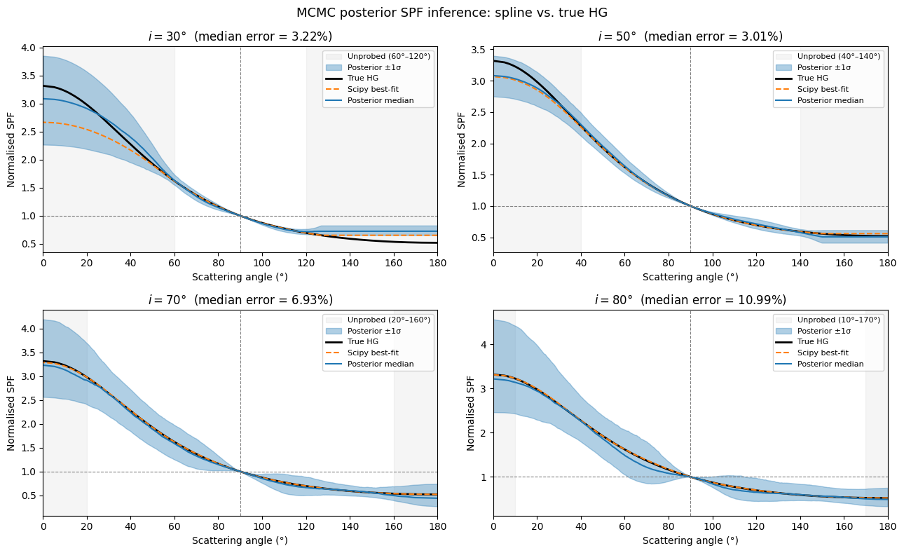
[12]:

# ── 2×2 MCMC posterior SPF panel ──────────────────────────────────────────────
fig, axes = plt.subplots(2, 2, figsize=(13, 8))

for ax, incl in zip(axes.flat, INCLINATIONS):
    r = mcmc_results[incl]
    cp_back, cp_fwd = r["cp_back"], r["cp_fwd"]
    ang_fwd  = float(np.degrees(np.arccos(cp_fwd)))
    ang_back = float(np.degrees(np.arccos(cp_back)))

    # Shade unprobed regions
    ax.axvspan(0,        ang_fwd,  alpha=0.08, color="grey")
    ax.axvspan(ang_back, 180,      alpha=0.08, color="grey",
               label=f"Unprobed ({ang_fwd:.0f}°–{ang_back:.0f}°)")

    ax.fill_between(angles, r["spf_lo"], r["spf_hi"],
                    alpha=0.35, color="C0", label="Posterior ±1σ")
    ax.plot(angles, r["true_spf_norm"],  "k-",  lw=2,   label="True HG")
    ax.plot(angles, r["recovered_spf"],  "--",  lw=1.5, color="C1", label="Scipy best-fit")
    ax.plot(angles, r["spf_median"],     "C0-", lw=1.5, label="Posterior median")

    ax.axvline(90, color="grey", ls="--", lw=0.8)
    ax.axhline(1.0, color="grey", ls="--", lw=0.8)

    ax.set_xlabel("Scattering angle (°)")
    ax.set_ylabel("Normalised SPF")
    ax.set_title(f"$i = {incl:.0f}$°  (median error = {r['max_frac_err_median']*100:.2f}%)")
    ax.legend(fontsize=8)
    ax.set_xlim(0, 180)

fig.suptitle("MCMC posterior SPF inference: spline vs. true HG", fontsize=13)
plt.tight_layout()
plt.show()

../_images/tutorials_spline_spf_tutorial_20_0.png

[13]:

# ── MCMC error summary table ──────────────────────────────────────────────────
print(f"{'Inclination':>12}  {'Mean |% diff|':>14}  {'Max |% diff|':>13}  {'Mean signed %':>14}")
print("-" * 60)
for incl in INCLINATIONS:
    r        = mcmc_results[incl]
    sr       = results[incl]
    in_range = sr["in_range"]
    true_v   = r["true_spf_norm"][in_range]
    med_v    = r["spf_median"][in_range]
    pct_diff = 100.0 * (med_v - true_v) / (np.abs(true_v) + 1e-30)
    mean_abs = float(np.mean(np.abs(pct_diff)))
    max_abs  = float(np.max(np.abs(pct_diff)))
    mean_sgn = float(np.mean(pct_diff))
    print(f"{incl:>11.0f}°  {mean_abs:>13.2f}%  {max_abs:>12.2f}%  {mean_sgn:>13.2f}%")

 Inclination   Mean |% diff|   Max |% diff|   Mean signed %
------------------------------------------------------------
         30°           1.10%          3.22%          -0.84%
         50°           1.12%          3.01%           0.95%
         70°           2.14%          6.93%          -1.92%
         80°           4.28%         10.99%          -3.99%

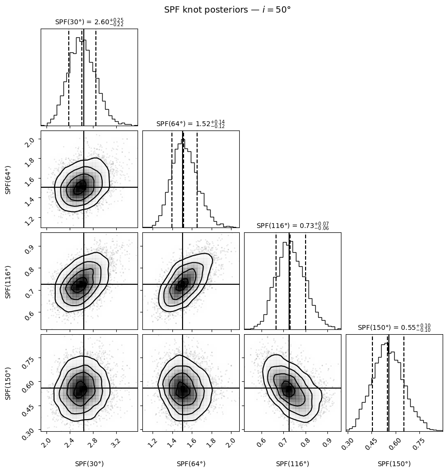
Corner Plots: SPF Knot Posteriors

A corner plot shows every pairwise marginal posterior distribution for the free parameters alongside the 1D marginals on the diagonal. It reveals:

Parameter uncertainty: wide marginals mean poorly constrained knots (typically near the edge of the probed range)
Correlations: off-diagonal structure shows which knot values are jointly constrained (adjacent knots often anti-correlate because they share leverage over the spline shape)
Accuracy: the black vertical/horizontal lines mark the true HG values; good recovery places the posterior peak on the truth

We show the posterior for $i = 50$°, which has clean, unimodal posteriors and is a representative case. The x-axis labels give the scattering angle for each free knot position.

[14]:

import corner

CORNER_INCL = 50.0   # inclination to show in the corner plot

r     = mcmc_results[CORNER_INCL]
sr    = results[CORNER_INCL]
nk    = r["nk"]
knots = np.array(r["knots"])

# Drop the fixed centre knot (index nk//2) to get only the free knot positions
n_left        = nk // 2
free_knot_cos = np.concatenate([knots[:n_left], knots[n_left + 1:]])
free_knot_ang = np.degrees(np.arccos(free_knot_cos))
labels        = [f"SPF({a:.0f}°)" for a in free_knot_ang]

# True HG values at each free knot position
truths = hg_normalized(free_knot_cos, G_TRUE)

# Subsample the chain for speed (corner is slow for > ~5000 points)
kv_samples = r["kv_samples"]
rng         = np.random.default_rng(42)
idx         = rng.choice(len(kv_samples), size=min(5000, len(kv_samples)), replace=False)
kv_sub      = kv_samples[idx]

fig = corner.corner(
    kv_sub,
    labels=labels,
    truths=truths,
    truth_color="k",
    show_titles=True,
    title_kwargs={"fontsize": 10},
    label_kwargs={"fontsize": 10},
    quantiles=[0.16, 0.5, 0.84],
    bins=30,
    smooth=1.0,
)
fig.suptitle(f"SPF knot posteriors — $i = {CORNER_INCL:.0f}$°", y=1.01, fontsize=13)
plt.show()

../_images/tutorials_spline_spf_tutorial_23_0.png

Summary

Recovery results

Inclination	Probed range	Knots	Scipy max err	MCMC median max err
30°	60° – 120°	4	0.09%	3.2%
50°	40° – 140°	4	0.68%	3.0%
70°	20° – 160°	6	0.61%	6.9%
80°	10° – 170°	6	1.01%	11.0%

Key takeaways

The spline SPF recovers a HG truth to <1% max error with scipy across all four inclinations in this test. The spline is flexible enough to represent the HG shape accurately within the probed range.
MCMC posteriors show 3–11% max error (median) with small mean bias (< 4%). The posterior median tracks the truth, and the ±1σ band spans the true HG curve in all cases. Larger uncertainty at $i = 80$° reflects the challenge of the narrow forward-scattering window, not a modelling failure.
The minimum reliable inclination is roughly 28°. Below this, the probed $\cos\phi$ window is too narrow to constrain the minimum of 4 free knots, leading to degenerate or locally-trapped fits. recommended_num_knots enforces a minimum of 4 for this reason.
``use_grad=False`` is faster for ~4–6 parameter fits. JAX JIT compilation overhead outweighs the benefit of autodiff gradients at this parameter scale. For larger models, use_grad=True wins decisively.
HG initialisation of the spline knots matters. Starting from a physically motivated forward-peaked shape prevents the optimiser from stalling in a flat-spline local minimum, especially at low inclinations where the gradient signal is weak.